Filter, Aggregate, and Export MCP Data Without Burning Context Tokens

You search LinkedIn for 200 software engineers. The MCP server fetches them. Then all 200 profiles — names, headlines, experience, follower counts, locations, skills — land in the LLM's context at once.

If you only wanted the ones in San Francisco with more than 500 followers, you still paid to load the other 170. If you wanted to know the average follower count by company, the LLM had to calculate that from raw data sitting in its context. At scale, this isn't just expensive. It's a structural ceiling.

The Anysite MCP Server v2 introduced a different model. Every execute() call stores results in a server-side data cache. Filtering, aggregation, and sorting happen server-side. Only the results you asked for come back to the LLM. The 200 profiles stay in the cache. What changes is how much of them you ever need to see.

The Context Window Tax

Context windows are finite. They're also shared. Every token spent holding raw data is a token unavailable for reasoning, instructions, and conversation history.

A single LinkedIn profile in structured JSON runs to roughly 800-1,500 tokens depending on how complete it is. Fetch 200 profiles and you've consumed somewhere between 160,000 and 300,000 tokens before asking a single question. For models with 200K token limits, that's most of the window. For models with smaller limits, it exceeds them entirely.

This shapes what you can do in a single MCP session. Want to compare follower counts across companies? The LLM reads each profile, extracts the follower count, holds all 200 numbers in working context, then calculates averages. It works. But you're using a language model as a spreadsheet, and paying language model prices to do it.

The bottleneck isn't intelligence. It's logistics.

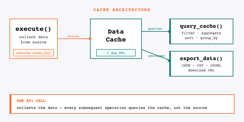
The Cache Architecture

Every execute() call automatically stores its results in a data cache on the Anysite servers. The call returns a cache_key — a reference to that stored dataset — along with the first page of results.

The cache persists for 7 days. During that time, query_cache and export_data can operate on the stored dataset without making new API requests and without returning all the raw data to the LLM.

execute() → stores to data cache → returns cache_key + first page
query_cache(cache_key, ...) → queries data cache → returns only results
export_data(cache_key, ...) → packages cached dataset → returns download URL

The distinction matters: query_cache is not re-fetching from LinkedIn or Twitter or wherever the data came from. It's querying an already-collected dataset that lives on Anysite's servers. One API call collects the data. Everything after that is analysis on the copy.

Filtering

The most common use case: collect broadly, then narrow down.

query_cache(cache_key, conditions=[
  {"field": "location", "op": "contains", "value": "San Francisco"},
  {"field": "followers", "op": ">", "value": 500}
])

This returns only profiles where location contains "San Francisco" and follower count exceeds 500. The rest of the dataset stays in the cache, untouched and unread.

Supported operators: =, !=, >, <, >=, <=, contains, not_contains. Multiple conditions use AND logic — every condition must match for a record to be included.

A few practical patterns:

Company filter: Find profiles from a specific employer.

{"field": "company", "op": "=", "value": "Anthropic"}

Exclusion filter: Remove records you don't want.

{"field": "industry", "op": "!=", "value": "Staffing and Recruiting"}

Keyword in text: Surface profiles mentioning a specific technology.

{"field": "headline", "op": "contains", "value": "machine learning"}

The filtered results come back to the LLM. The discarded records do not.

Aggregation

Aggregation answers analytical questions about a dataset without requiring the LLM to hold the dataset in context.

Average follower count across all collected profiles:

query_cache(cache_key, aggregate={"field": "followers", "op": "avg"})

Supported functions: sum, avg, min, max, count, uniq.

count returns the total number of records in the dataset. uniq counts distinct values in a field — useful for understanding how many unique companies, locations, or industries appear in a dataset.

None of these operations require the LLM to see individual records. The calculation runs server-side. The LLM receives a single number.

Group By

Group by lets you break aggregations down by a categorical field. The pattern: aggregate a metric, grouped by a dimension.

Average follower count broken down by company:

query_cache(cache_key,
  aggregate={"field": "followers", "op": "avg"},
  group_by="company"
)

Count of profiles by industry:

query_cache(cache_key,
  aggregate={"field": "followers", "op": "count"},
  group_by="industry"
)

The result is a table: one row per unique value of the group-by field, with the aggregate value for each group. You can group by any field in the dataset — location, seniority, company size, or any other structured attribute in the response.

This is the difference between "how many profiles did we collect?" and "how are those profiles distributed across industries?" Both questions answer from the same cache. Neither requires loading the full dataset.

Sorting and Pagination

Sort by any field in the dataset, with an optional limit:

query_cache(cache_key, sort_by="followers", sort_order="desc", limit=10)

This returns the 10 profiles with the highest follower counts. The LLM sees 10 records, not 200.

Combine sorting with filtering to get precise subsets:

query_cache(cache_key,
  conditions=[{"field": "location", "op": "contains", "value": "New York"}],
  sort_by="followers",
  sort_order="desc",
  limit=20
)

Top 20 most-followed profiles in New York, from a 200-profile dataset. Two conditions applied server-side. Twenty records returned to context.

For large result sets, use get_page to paginate through cached results:

get_page(cache_key, offset=20)

A Complete Workflow

Here's how the pieces fit together in practice. The goal: find the most-followed ML engineers in the Bay Area from a broad LinkedIn search, then export the full filtered dataset for a spreadsheet.

Step 1: Collect broadly.

execute("linkedin", "user", "search", {"keywords": "machine learning engineer", "limit": 200})

Returns cache_key + first 10 profiles. 200 profiles now in the data cache.

Step 2: Filter to Bay Area.

query_cache(cache_key, conditions=[
  {"field": "location", "op": "contains", "value": "Bay Area"}
])

Returns the subset of Bay Area profiles. No new API call. No re-fetching from LinkedIn.

Step 3: Check the distribution.

query_cache(cache_key,
  aggregate={"field": "followers", "op": "count"},
  group_by="current_company"
)

Reveals which companies have the most ML engineers in the dataset.

Step 4: Get the top 15 by follower count.

query_cache(cache_key,
  conditions=[{"field": "location", "op": "contains", "value": "Bay Area"}],
  sort_by="followers",
  sort_order="desc",
  limit=15
)

Fifteen profiles, sorted. Ready to read.

Step 5: Export the full Bay Area subset.

export_data(cache_key, "csv")

All five steps operate on the same collected dataset. One API call to LinkedIn. The rest is analysis.

Exporting Datasets

export_data packages the full cached dataset as a downloadable file. Three formats: JSON, CSV, and JSONL.

export_data(cache_key, "csv")

The tool returns a download URL. The file stays available for 7 days — the same TTL as the cache. Download it into a spreadsheet, load it into a database, pass the URL to a reporting tool.

CSV works for spreadsheets and most BI tools. JSON preserves nested data structures from the original response. JSONL (newline-delimited JSON) works best for large datasets that need to be processed line by line or streamed into a database.

Exporting is particularly useful when analysis needs to exceed what any MCP session can handle. A 200-profile dataset in a spreadsheet can be filtered, pivoted, and charted without token constraints.

Best Practices

Collect broadly, filter narrowly. Use larger count values in execute() — the cache is cheap. Filtering server-side is cheaper than making multiple narrow API calls, and you can slice the same dataset multiple ways without re-collecting.

Filter before reading into context. If you know you only want a subset of a dataset, apply query_cache before asking the LLM to analyze individual records. There's no reason to load 200 records when you want 15.

Aggregate server-side. If the question is statistical — averages, counts, distributions — let the server calculate it. The LLM receives a number, not a dataset.

Export for external analysis. When the analysis requires a tool better suited to tabular data — a spreadsheet, a SQL query, a BI dashboard — export the dataset and work there. The MCP session is for discovery and exploration, not for being a calculation engine.

Know when to graduate. MCP is built for exploration: ad-hoc queries, conversational analysis, one-off research. When a workflow becomes routine — weekly competitive reports, daily prospect refreshes, ongoing talent pipeline tracking — it belongs in the CLI as a scheduled pipeline. The same Anysite engine powers both. The difference is the interface and whether a human needs to be involved.

What This Changes

The practical effect of server-side analysis is that the size of a dataset stops being the constraint on what you can analyze. You can collect 500 records, filter to 30, aggregate across all 500, and export the full set — in the same session, from the same cache.

Context windows expand over time. But the architectural principle holds regardless: analysis that runs on the data source is more efficient than analysis that requires the data to travel through context. For data-heavy MCP workflows, query_cache is the difference between what fits and what doesn't.

Full documentation for query_cache and export_data is at docs.anysite.io.